代谢组学常用仪器特点
| 仪器 | 特点 |
|---|---|
| GC-MS | 易挥发,低极性,热稳定的小分子化合物;需衍生化 |
| LC-MS | 具有一定极性的有机化合物;无需衍生化 |
| NMR | 无偏性,无损检测;•无需繁琐前处理,便于活体、原位的动态检测 |
| CE-MS | 高极性化合物,如核酸,蛋白等 |
| ICP-MS | 无机化合物 |
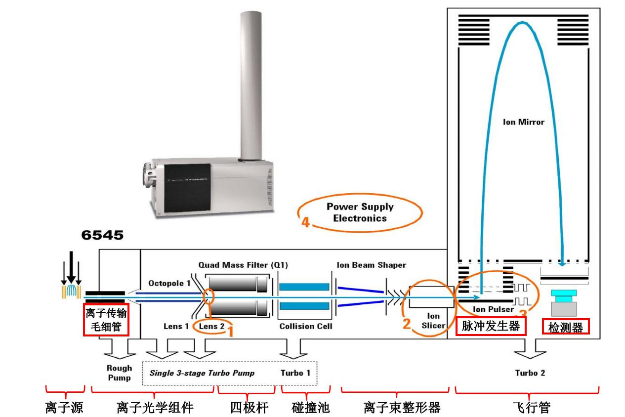
LC-QTOF原理
Q-TOF全称为四极飞行时间质谱仪(Quadrupole Time-of-Flight Mass Spectrometer)。其基本原理是将样品离子通过四极杆进行质量筛选,然后进入飞行时间质谱器(Time-of-Flight Mass Analyzer,ToF),测定其离子的飞行时间,从而得到样品中离子的质量信息。Q-TOF有正离子模式(positive ion mode, POS)和负离子模式(negative ion mode, NEG)两种电离方式,在检测代谢组时结合使用两种方式可以使代谢物覆盖率更高,检测效果也更好。
Q-TOF的工作过程包含以下步骤:
离子化:样品通过电喷雾或者MALDI等方法被电离成为离子。
生成离子束:离子经过引出阱、加速器、光栅偏转镜等装置,形成一个带电的离子束。
四极杆质量筛选:离子束进入四极杆,通过高频交变电压(RF)和直流电压(DC)的控制,将不同质量的离子分离出来。
飞行时间质谱分析:通过激光或者其他方法对分散的离子束施加助推、聚焦和分析,并且测定其到达检测器所需的时间。不同质量的离子抵达检测器所需要的时间不同,从而可以得到离子的质量信息。
FAQ:POS和NEG数据的利用。
负离子和正离子是数据采集时的时候的两种模式生成两套数据,一级分析(MS)结果中是提供 POS 和 NEG 两个检测结果列表的,但是在二级分析(MSMS)结果中,我们将鉴定正负离子模式下鉴定到的物质进行了合并,所以二级分析是针对代谢物来做的,不区分正负离子模式。
FAQ: 当正负离子模式下都检测到了某种物质,如何对该物质的结果进行呈现?
会根据匹配参数进行取舍,选用匹配参数更好的模式下的数据在二级结果中进行分析。
数据分析
下机数据格式转换
以下两个软件二选一,Windows下建议使用ProteoWizard,其用法可参考用metid构建代谢组数据库。Linux下建议使用massconverter。
ProteoWizard
将raw data转换为mzXML格式。
massconverter
将raw data转换为mzXML格式。
安装
1 | if(!require(remotes)){ |
Debug:如果报错Error in docker_pull_pwiz() : Please install docker first (https://www.docker.com/get-started),则首先确认系统是否已安装docker,如果未安装,请先安装docker;如已经安装,则是因为普通用户无运行docker的权限,将其添加到docker用户组中即可。
1 | root模式下运行如下shell命令,将用户lhl添加到docker组中 |
设置转换参数
此处调用MSConvert进行格式转换,期间进行了过滤,主要采用了Peak Picking,Subset,和Zero Samples方法。
1 | parameter = |
开始转换
1 | convert_raw_data(input_path = "demo_data/raw_data", |
安装tidyMass
1 | mamba install gcc_linux-64 gxx_linux-64 gfortran_linux-64 |
1 | if(!require(remotes)){ |
原始数据处理
调用massprocesser包进行原始数据处理,进行峰检测与对齐,输出peak table包括:
原始数据导入(read spectra from file)、峰检测(detect mass traces & detect chromatographic peaks)、校正保留时间(Correcting rentention time)、对已鉴定的色谱峰进行保留时间校正、Grouping peaks across samples、输出peak table。
数据目录结构
- mzxml/mzxml_ms1_data/
- POS/
- Case/*.mzXML
- Control/*.mzXML
- QC/*.mzXML
- NEG/
- Case/*.mzXML
- Control/*.mzXML
- QC/*.mzXML
- POS/
- mzxml/mgf_ms2_data/mgf_ms2_data/
- POS/*.mgf
- NEG/*.mgf
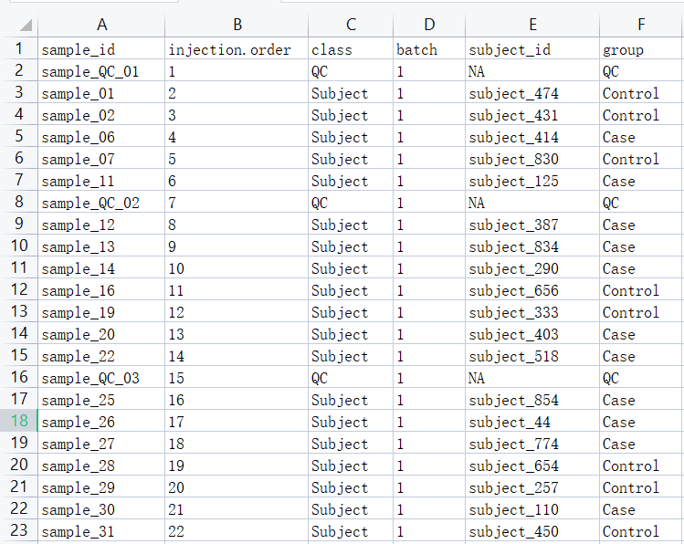
- mzxml/sample_info/
- sample_info_pos.csv
- sample_info_neg.csv
正离子模式
注意:path指定的路径名不可以数字开头!
1 | library(tidymass) |
- ppm:numeric defining the maximal tolerated m/z deviation in consecutive scans in parts per million (ppm) for the initial regions-of-interest (ROI) definition。此处的ppm来源于xcms包,但在xcms中不同的函数中,含义貌似不一样,需进一步确认。
- peakwith:峰宽,取决于柱子(column)和LC系统。numeric(2) with the expected approximate peak width in chromatographic space. Given as a range (min, max) in seconds.
- min_fraction:如果一个峰出现在至少一组样本中
min_fraction样本以上(按比例),则将保留该峰值。 - snthresh :信噪比阈值。
- prefilter:c(k, I) 在第一次分析步骤(ROI检测)中指定预筛选步骤。仅保留包含至少强度>=I的k个峰的的质量轨迹(Mass traces)。
- fitgauss :是否应对每个峰拟合高斯分布。主要影响峰的保留时间位置。
- integrate:积分方法(1或2)。对于 integrate=1,Peak limits通过在mexican hat 过滤后的数据上下降(descent)来确定;而对于 integrate=2,则在原始数据上进行下降处理。后一种方法更准确但容易受到噪声的影响,而前一种方法更稳健但不太精确。
- mzdiff :representing the minimum difference in m/z dimension required for peaks with overlapping retention times; can be negative to allow overlap. During peak post-processing, peaks defined to be overlapping are reduced to the one peak with the largest signal.
- noise:设定第一步分析中需要的质心(centroids )最小强度(intensity < noise的质心将被省略在感兴趣区域检测之外)。
- binSize :将m/z轴按照binSize划分为多个区间,再对各区间内的离子信号进行聚合。较小的binSize使得峰检测更加准确,检测到更多features,需要更多计算资源。
- bw:带宽,通常在5-50间,这是用于峰值检测的核密度估计 (KDE) 算法中使用的参数。bw 控制估计的 KDE 曲线的平滑度,并确定峰的解析程度。较小的bw值将产生更详细的基础峰形表示,在紧密间隔或重叠的峰之间具有更好的分辨率,但也可能产生更高水平的噪声。相反,较大的bw值将导致对峰形的估计更平滑、更广义,这有助于降低噪声和杂散检测,但在某些情况下也可能导致峰分辨率降低。bw 值的选择将取决于所分析数据的具体特征以及分析的目标。通常,有必要试验一系列 bw 值,以找到给定数据集的最佳设置。
- fill_peaks:Fill peaks NA or not。
结果:
POS/Result/
object:用于下一步分析
Peak_table.csv:用于下一步分析的峰表
Peak_table_for_cleaning.csv:删除了
Peak_table.csv中无用的列,可直接用于后续的数据清洗BPC.pdf:Base peak chromatogram,仅展示
group_for_figure参数指定组内的样本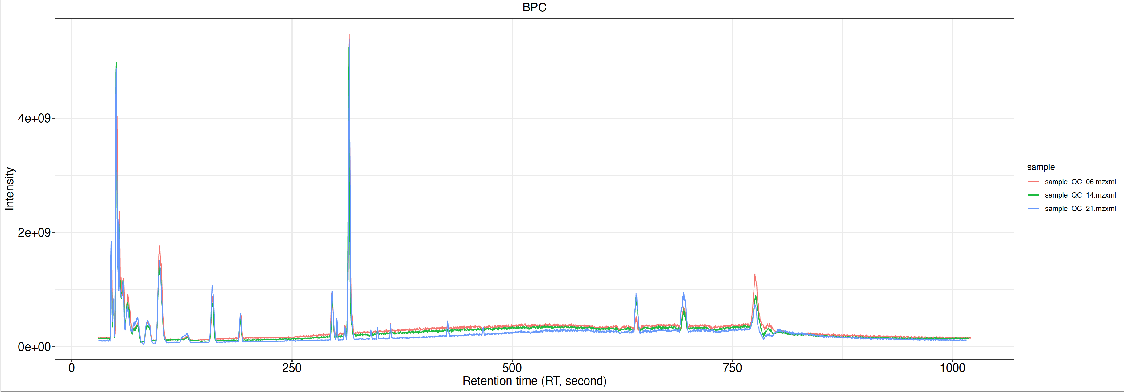
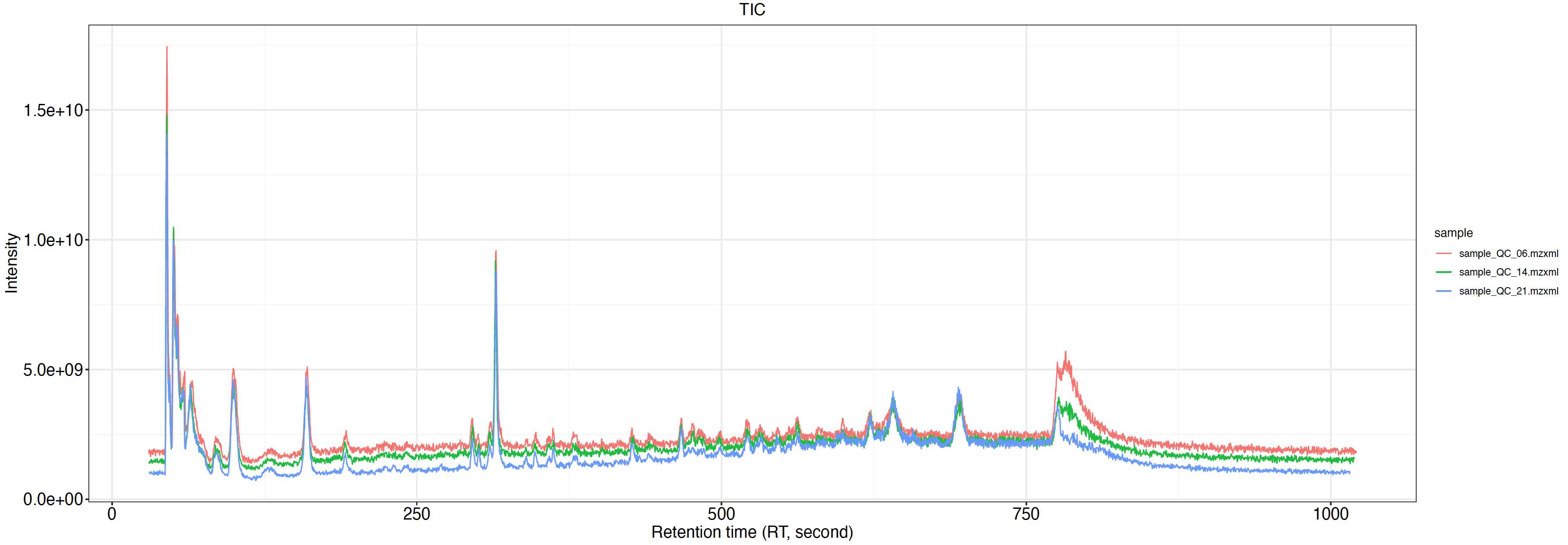
TIC.pdf:Total ion peak chromatogram,经色谱分离流出的组分不断进入质谱,质谱连续扫描采集数据,每一次扫描得到一张质谱图,将每一张质谱图中所有离子强度相加得到总离子流强度。然后以总离子强度为纵坐标,时间为横坐标绘图。
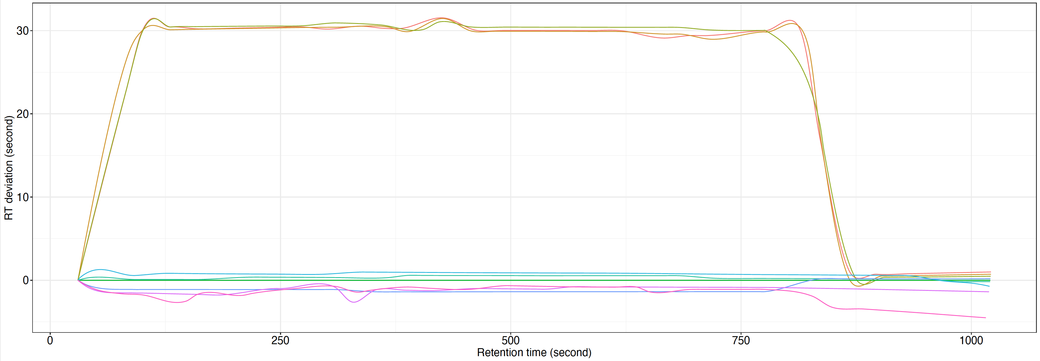
RT correction plot.pdf
intermediate_data:中间文件目录,如果需要重新运行data processing,则需先删除该目录。
1
2
3
4
5
6
7
8
9
10
11
12# 加载对象
load("mzxml_ms1_data/POS/Result/object")
# 查看metabolic features数量
object
# 获取互动图,在Rstudio中才能显示
load("mzxml_ms1_data/POS/Result/intermediate_data/xdata2")
plot = massprocesser::plot_adjusted_rt(object = xdata2, group_for_figure = "QC", interactive = TRUE)
plot
负离子模式
1 | massprocesser::process_data( |
1 | # 加载对象 |
Explore data
将peak table和样本信息(元数据)整合,得到mass_dataset class对象。获取数据的总结信息。
1 | library(tidyverse) |
正离子模式
1 | # 加载对象 |
1 | # 统计样本数和variables数 |

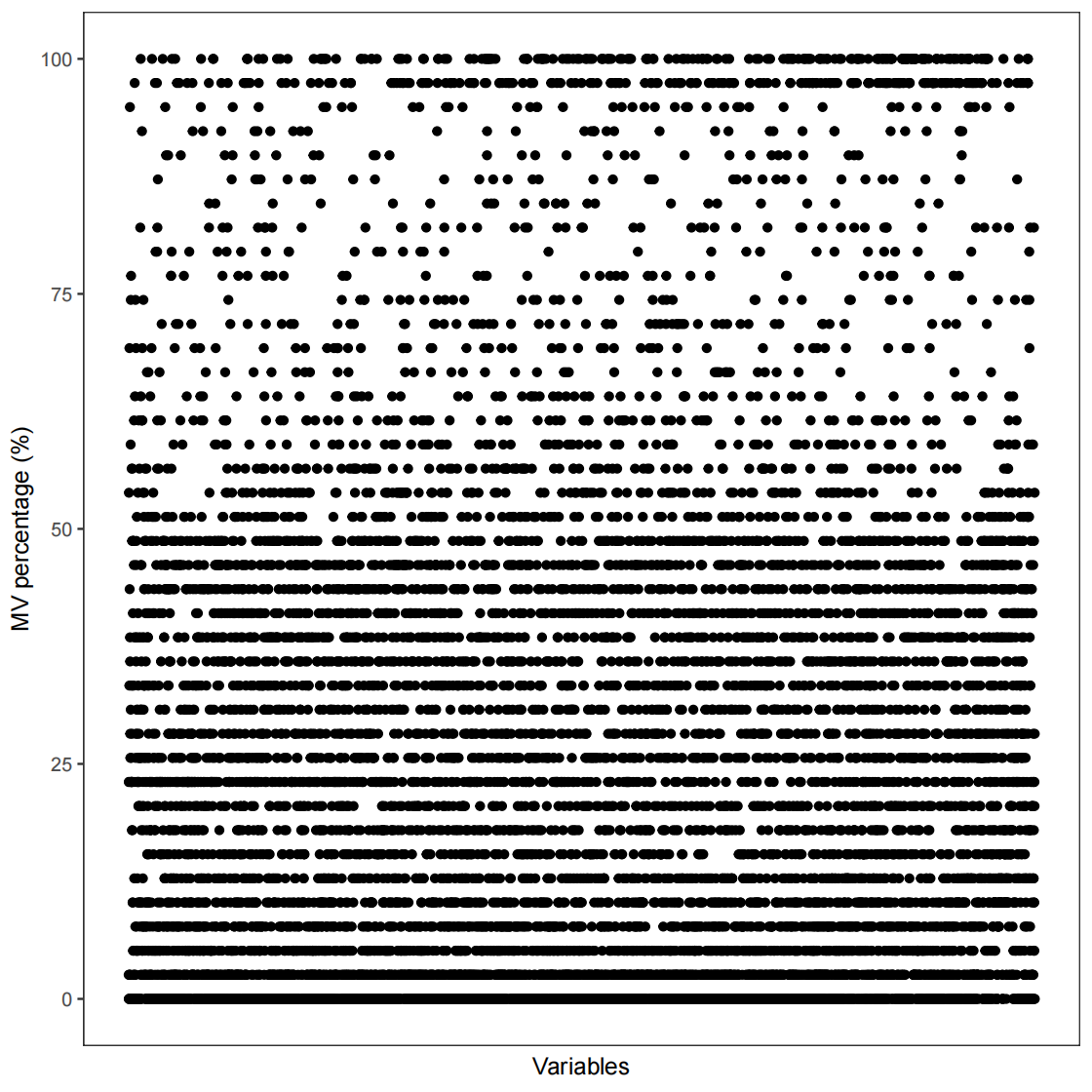
黑色代表缺失值。


负离子模式
1 | # 加载对象 |
1 | # 统计样本数和variables数 |
数据清洗(Data cleaning)
查看质量
1 | # 加载数据 |
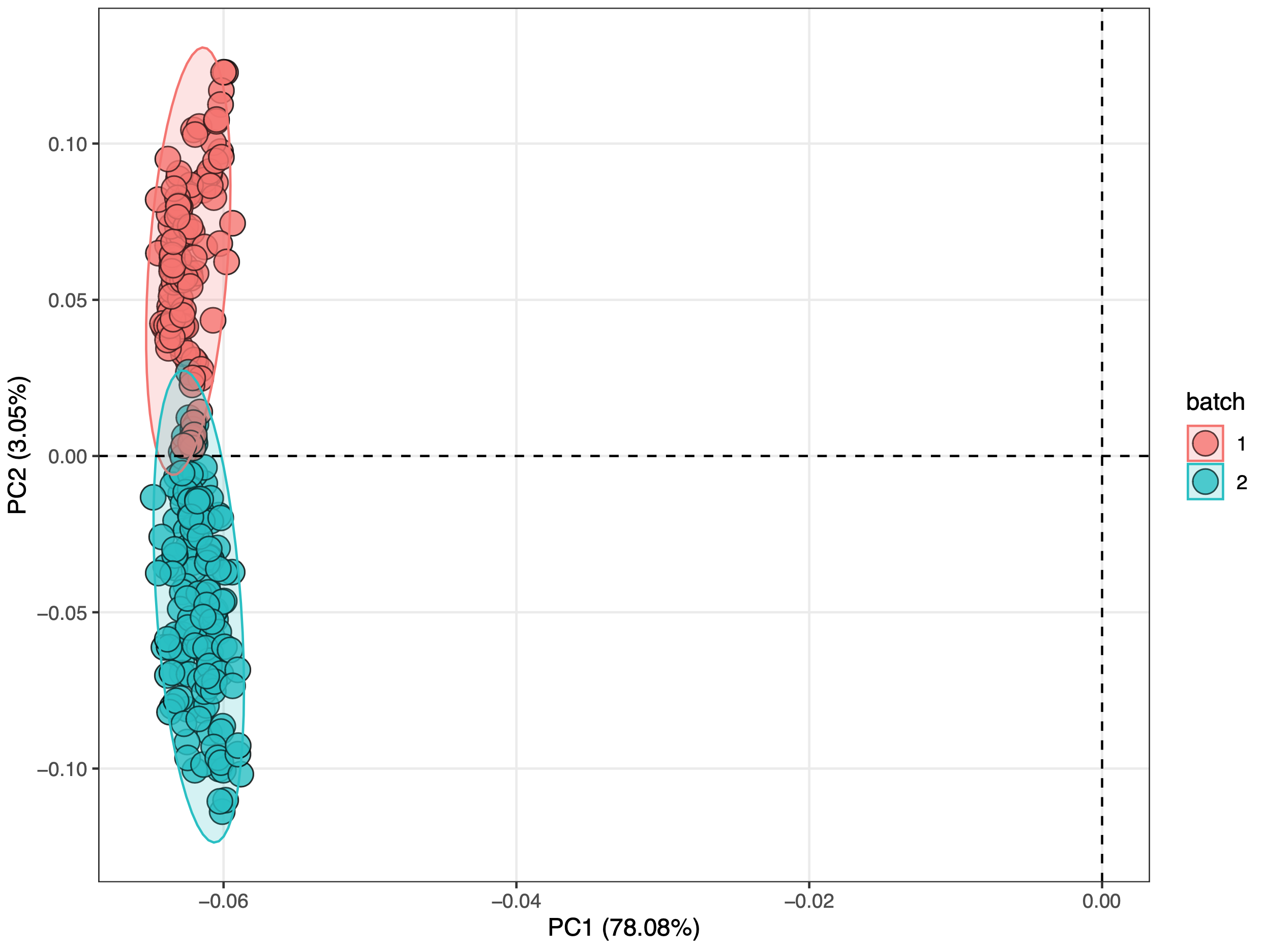
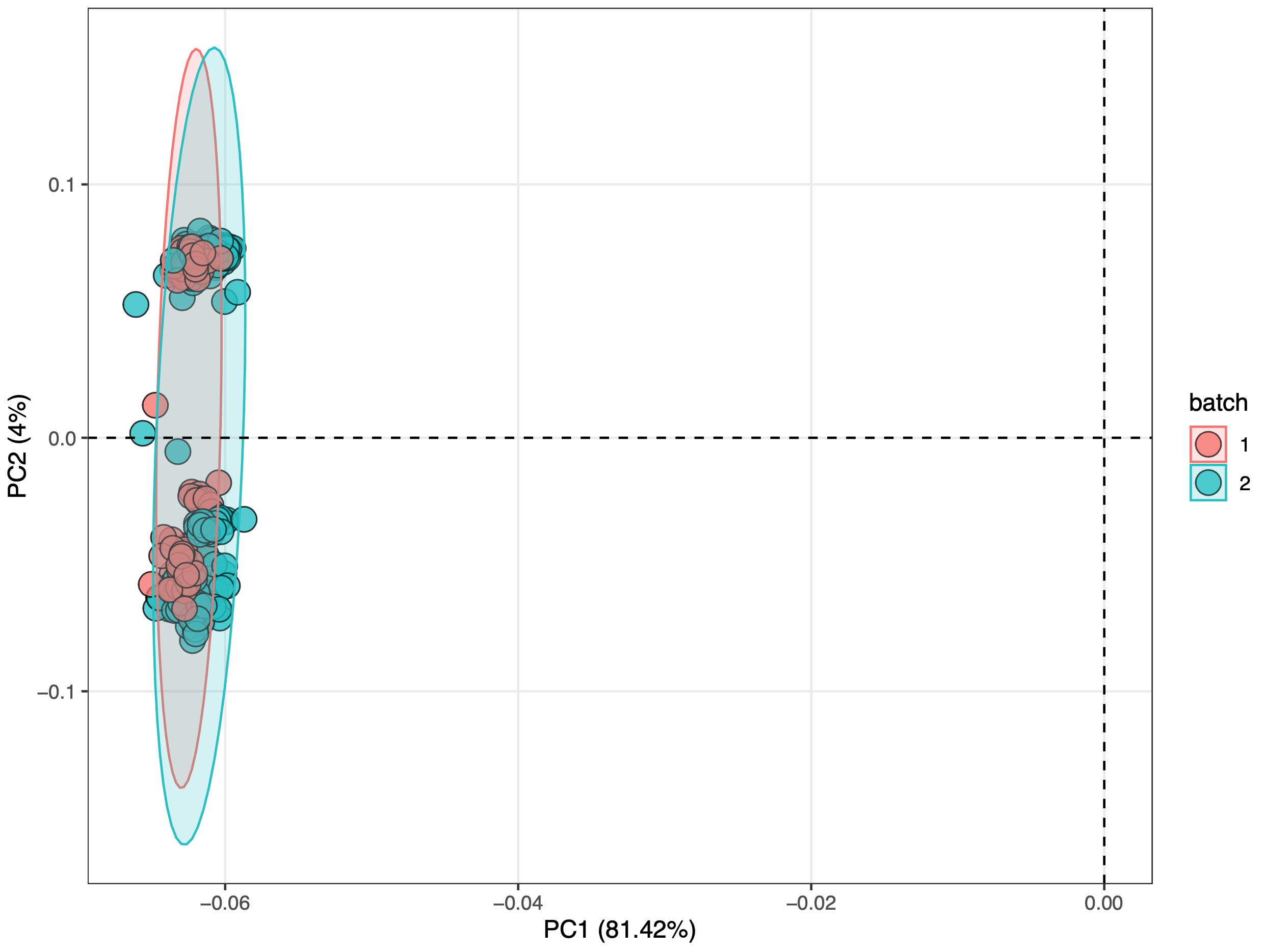
从上两图可看出正离子模式下存在严重的批次效应,负离子模式下不存在明显的批次效应。
开始清洗
移除噪音代谢features——缺失值过滤。
移除超过20% QC样本中含有MVs以及至少在50%实验组或对照组样本中含有MVs的variables。
正离子模式
1
2
3
4
5
6
7
8
9
10
11
12
13
14
15
16
17
18
19
20
21
22
23
24
25
26
27
28
29
30
31
32
33
34
35
36
37
38
39
40
41# 查看各分组样本量
object_pos %>% activate_mass_dataset(what = "sample_info") %>% dplyr::count(group)
#> group n
#> 1 Case 110
#> 2 Control 110
#> 3 QC 39
# QC样本中的MV占比
pdf(file="data_cleaning/POS/MVpercentQC.pdf")
p<- show_variable_missing_values(object = object_pos %>% activate_mass_dataset(what = "sample_info") %>% filter(class == "QC"), percentage = TRUE)
p+ scale_size_continuous(range = c(0.01, 2))
dev.off()
# 统计QC中的MV占比
qc_id = object_pos %>% activate_mass_dataset(what = "sample_info") %>% filter(class == "QC") %>% pull(sample_id)
# 统计对照组中的MV占比
control_id = object_pos %>% activate_mass_dataset(what = "sample_info") %>% filter(group == "Control") %>% pull(sample_id)
# 统计实验组中的MV占比
case_id = object_pos %>% activate_mass_dataset(what = "sample_info") %>% filter(group == "Case") %>% pull(sample_id)
# 整合以上统计信息
object_pos = object_pos %>% mutate_variable_na_freq(according_to_samples = qc_id) %>% mutate_variable_na_freq(according_to_samples = control_id) %>% mutate_variable_na_freq(according_to_samples = case_id)
head(extract_variable_info(object_pos))
#variable_id mz rt na_freq na_freq.1 na_freq.2
#1 M70T73_POS 70.04074 73.31705 0.28205128 0.6000000 0.4727273
#2 M70T53_POS 70.06596 52.78542 0.00000000 0.1454545 0.0000000
#3 M70T183_POS 70.19977 182.87981 0.00000000 0.6636364 0.7454545
#4 M70T527_POS 70.36113 526.76657 0.02564103 0.1818182 0.3000000
#5 M71T695_POS 70.56911 694.84592 0.02564103 0.6454545 0.5545455
#6 M71T183_POS 70.75034 182.77790 0.05128205 0.7272727 0.7909091
# 移除variables
object_pos <- object_pos %>% activate_mass_dataset(what = "variable_info") %>% filter(na_freq < 0.2 & (na_freq.1 < 0.5 | na_freq.2 < 0.5))
object_pos注:na_freq、na_freq.1和na_freq.2在此处分别代表某variables 在QC样本、对照组样本和实验组样本中缺失值MV所占的百分比。
负离子模式
1
2
3
4
5
6
7
8
9
10
11
12
13
14
15
16
17
18
19
20
21
22
23
24
25
26
27
28
29
30
31
32
33
34
35
36
37
38
39
40
41# 查看各分组样本量
object_neg %>% activate_mass_dataset(what = "sample_info") %>% dplyr::count(group)
#> group n
#> 1 Case 110
#> 2 Control 110
#> 3 QC 39
# QC样本中的MV占比
pdf(file="data_cleaning/NEG/MVpercentQC.pdf")
p<- show_variable_missing_values(object = object_neg %>% activate_mass_dataset(what = "sample_info") %>% filter(class == "QC"), percentage = TRUE)
p+ scale_size_continuous(range = c(0.01, 2))
dev.off()
# 统计QC中的MV占比
qc_id = object_neg %>% activate_mass_dataset(what = "sample_info") %>% filter(class == "QC") %>% pull(sample_id)
# 统计对照组中的MV占比
control_id = object_neg %>% activate_mass_dataset(what = "sample_info") %>% filter(group == "Control") %>% pull(sample_id)
# 统计实验组中的MV占比
case_id = object_neg %>% activate_mass_dataset(what = "sample_info") %>% filter(group == "Case") %>% pull(sample_id)
# 整合以上统计信息
object_neg = object_neg %>% mutate_variable_na_freq(according_to_samples = qc_id) %>% mutate_variable_na_freq(according_to_samples = control_id) %>% mutate_variable_na_freq(according_to_samples = case_id)
head(extract_variable_info(object_neg))
#variable_id mz rt na_freq na_freq.1 na_freq.2
#1 M70T712_NEG 70.05911 711.97894 0.05128205 0.109090909 0.018181818
#2 M70T527_NEG 70.13902 526.85416 0.33333333 0.509090909 0.618181818
#3 M70T587_NEG 70.31217 587.25330 0.00000000 0.009090909 0.009090909
#4 M70T47_NEG 70.33835 46.57537 0.84615385 0.936363636 0.090909091
#5 M71T587_NEG 70.56315 587.02570 0.17948718 0.145454545 0.163636364
#6 M71T641_NEG 70.70657 641.16672 0.10256410 0.063636364 0.072727273
# 移除variables
object_neg <- object_neg %>% activate_mass_dataset(what = "variable_info") %>% filter(na_freq < 0.2 & (na_freq.1 < 0.5 | na_freq.2 < 0.5))
object_neg
过滤离群样本(Filter outlier samples)
正离子模式
1
2
3
4
5
6
7
8
9
10
11
12
13
14
15
16
17
18
19
20
21
22
23
24
25
26
27
28
29
30
31
32
33
34
35# 总览
pdf(file="data_cleaning/POS/MVpercentALL.pdf")
massdataset::show_sample_missing_values(object = object_pos, color_by = "group", order_by = "injection.order", percentage = TRUE) + theme(axis.text.x = element_text(size = 2)) + scale_size_continuous(range = c(0.1, 2)) + ggsci::scale_color_aaas()
dev.off()
# 检测离群样本
outlier_samples = object_pos %>% `+`(1) %>% log(2) %>% scale() %>% detect_outlier()
outlier_samples
#--------------------
#masscleaner
#--------------------
#1 according_to_na : 0 outlier samples.
#2 according_to_pc_sd : 0 outlier samples.
#3 according_to_pc_mad : 0 outlier samples.
#4 accordint_to_distance : 0 outlier samples.
#4 accordint_to_distance : 0 outlier samples.
#extract all outlier table using extract_outlier_table()
outlier_table <- extract_outlier_table(outlier_samples)
outlier_table %>% head()
# according_to_na pc_sd pc_mad accordint_to_distance
#sample_06 FALSE FALSE FALSE FALSE
#sample_103 FALSE FALSE FALSE FALSE
#sample_11 FALSE FALSE FALSE FALSE
#sample_112 FALSE FALSE FALSE FALSE
#sample_117 FALSE FALSE FALSE FALSE
#sample_12 FALSE FALSE FALSE FALSE
outlier_table %>% apply(1, function(x){ sum(x) }) %>% `>`(0) %>% which()
# #named integer(0)
##无离群样本1
2
3
4# 删除离群样本,如果有的话
need_id_pos <- names(outlier_table %>% apply(1, function(x){ sum(x) }) %>% `==`(0) %>% which())
object_pos <- object_pos %>% activate_mass_dataset(what = "sample_info") %>% filter(sample_id %in% need_id_pos)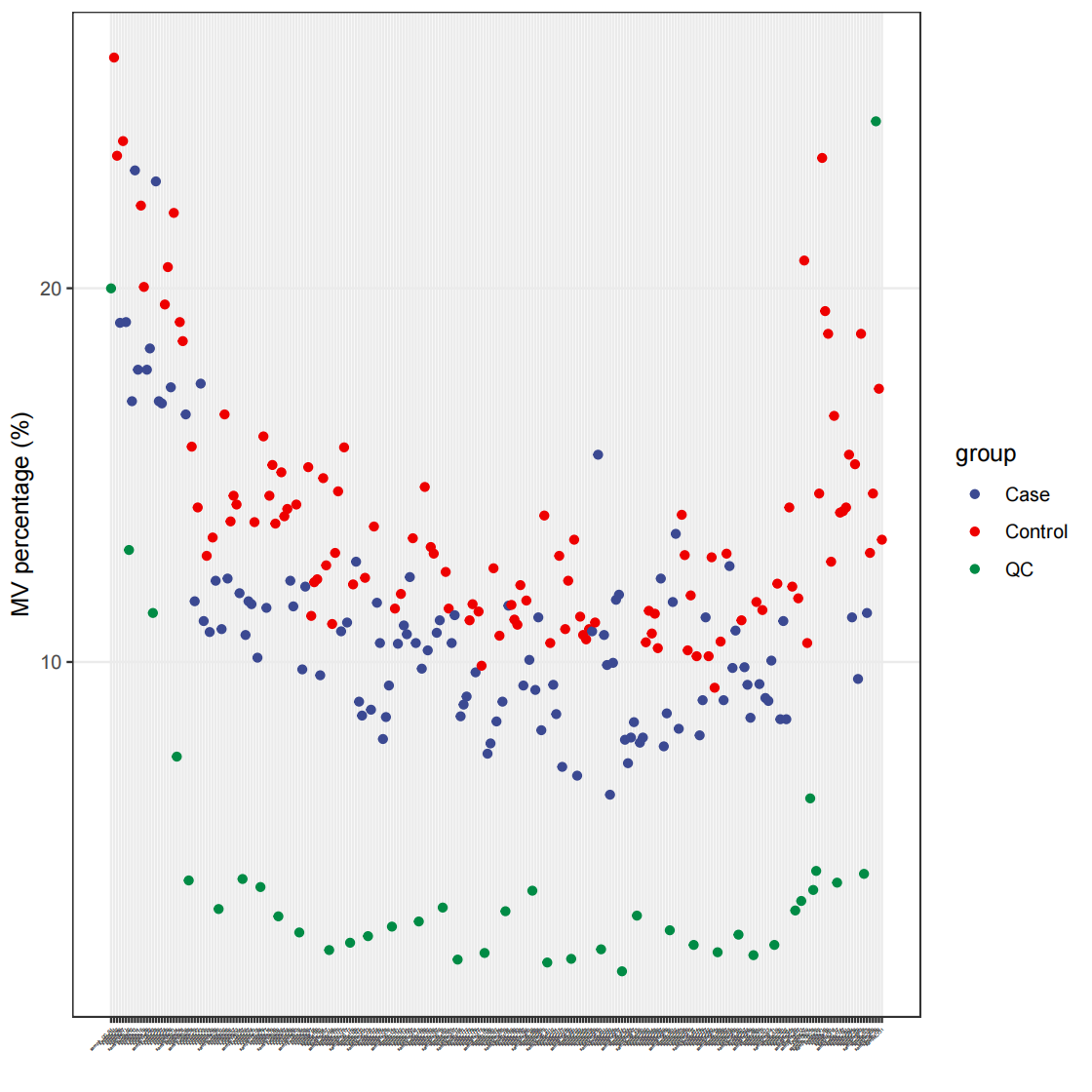
负离子模式
1
2
3
4
5
6
7
8
9
10
11
12
13
14
15
16
17
18
19
20
21
22
23
24
25
26
27
28
29
30
31
32
33
34
35
36
37# 总览
pdf(file="data_cleaning/NEG/MVpercentALL.pdf")
p<- massdataset::show_sample_missing_values(object = object_neg, color_by = "group", order_by = "injection.order", percentage = TRUE)
p+ theme(axis.text.x = element_text(size = 2)) + scale_size_continuous(range = c(0.1, 2)) + ggsci::scale_color_aaas()
dev.off()
# 检测离群样本
outlier_samples = object_neg %>% `+`(1) %>% log(2) %>% scale() %>% detect_outlier()
outlier_samples
#--------------------
#masscleaner
#--------------------
#1 according_to_na : 0 outlier samples.
#2 according_to_pc_sd : 0 outlier samples.
#3 according_to_pc_mad : 0 outlier samples.
#4 accordint_to_distance : 0 outlier samples.
#4 accordint_to_distance : 0 outlier samples.
#extract all outlier table using extract_outlier_table()
outlier_table <- extract_outlier_table(outlier_samples)
outlier_table %>% head()
# according_to_na pc_sd pc_mad accordint_to_distance
#sample_06 FALSE FALSE FALSE FALSE
#sample_103 FALSE FALSE FALSE FALSE
#sample_11 FALSE FALSE FALSE FALSE
#sample_112 FALSE FALSE FALSE FALSE
#sample_117 FALSE FALSE FALSE FALSE
#sample_12 FALSE FALSE FALSE FALSE
outlier_table %>% apply(1, function(x){ sum(x) }) %>% `>`(0) %>% which()
# #named integer(0)
##无离群样本
缺失值填充(Missing value imputation)
对原始数据中的缺失值进行模拟(missing value recoding)。方法包括:”knn”, “rf” (missForest), “mean”, “median”, “zero”, “minimum”, “bpca”, “svdImpute”, “ppca”。
1 | # 获取正离子模式下的MV数量 |
数据标准化与整合(Data normalization and integration)
数据标准化处理, 利用内标(internal standard, IS)进行归一化待确认是否通过IS实现。
正离子模式
标准化方法包括:”svr”, “total”, “median”, “mean”, “pqn”, “loess”;整合方法包括:”qc_mean”, “qc_median”, “subject_mean”, “subject_median”。
1
2
3
4
5
6
7
8
9
10object_pos <- normalize_data(object_pos, method = "median")
object_pos2 <- integrate_data(object_pos, method = "subject_median")
# 按批次分组绘制PCA图
pdf(file="data_cleaning/POS/PC_batch_intergrated.pdf")
object_pos2 %>% `+`(1) %>% log(2) %>% massqc::massqc_pca(color_by = "batch", line = FALSE)
dev.off()

负离子模式
1
2
3
4
5
6
7
8
9
10object_neg <- normalize_data(object_neg, method = "median")
object_neg2 <- integrate_data(object_neg, method = "subject_median")
# 按批次分组绘制PCA图
pdf(file="data_cleaning/NEG/PC_batch_intergrated.pdf")
object_neg2 %>% `+`(1) %>% log(2) %>% massqc::massqc_pca(color_by = "batch", line = FALSE)
dev.off()

保存数据
1 | save(object_pos2, file = "data_cleaning/POS/object_pos2") |
代谢物注释
加载数据
1 | load("data_cleaning/POS/object_pos2") |
将MS2数据添加到mass_dataset
如果没有MS2数据,此步不执行应该也可以!
??只有QC样的MS2数据,MS2数据是怎么来的?
正离子模式
1
2
3
4
5
6
7
8
9
10
11
12
13object_pos2 <- mutate_ms2(
object = object_pos2,
column = "rp", # rp or hilic,对应RPLC(反相色谱)和HILIC(亲水相互作用色谱)
polarity = "positive",
ms1.ms2.match.mz.tol = 15,# ppm
ms1.ms2.match.rt.tol = 30,# seconds
path = "mgf_ms2_data/mgf_ms2_data/POS"
)
#1043 out of 5101 variable have MS2 spectra.
#Selecting the most intense MS2 spectrum for each peak...
# summary
extract_ms2_data(object_pos2)负离子模式
1
2
3
4
5
6
7
8
9
10
11
12
13object_neg2 <- mutate_ms2(
object = object_neg2,
column = "rp",
polarity = "negative",
ms1.ms2.match.mz.tol = 15,
ms1.ms2.match.rt.tol = 30,
path = "mgf_ms2_data/mgf_ms2_data/NEG"
)
#1092 out of 4104 variable have MS2 spectra.
#Selecting the most intense MS2 spectrum for each peak...
# summary
extract_ms2_data(object_neg2)
代谢物注释
需要考虑数据库是RPLC还是HILIC。
正离子模式
1
2
3
4
5
6
7
8
9
10
11
12
13
14
15
16
17
18
19
20
21
22
23
24
25
26
27
28
29
30
31
32
33
34
35
36
37
38
39
40
41
42# Annotate features using snyder_database_rplc0.0.3
load("metabolite_annotation/snyder_database_rplc0.0.3.rda")
## 查看数据库信息
snyder_database_rplc0.0.3
## 注释
object_pos2 <- annotate_metabolites_mass_dataset(
object = object_pos2,
ms1.match.ppm = 15,
rt.match.tol = 30,
polarity = "positive",
database = snyder_database_rplc0.0.3,
threads =30)
# Annotate features using orbitrap_database0.0.3
load("metabolite_annotation/orbitrap_database0.0.3.rda")
## 查看数据库信息
orbitrap_database0.0.3
## 注释
object_pos2 <- annotate_metabolites_mass_dataset(
object = object_pos2,
ms1.match.ppm = 15,
polarity = "positive",
database = orbitrap_database0.0.3,
threads =30)
# Annotate features using mona_database0.0.3
load("metabolite_annotation/mona_database0.0.3.rda")
## 查看数据库信息
mona_database0.0.3
## 注释
object_pos2 <- annotate_metabolites_mass_dataset(
object = object_pos2,
ms1.match.ppm = 15,
polarity = "positive",
database = mona_database0.0.3,
threads =30)annotate_metabolites_mass_dataset 参数解析:
- ms1.match.ppm:Precursor match ppm tolerance [25].
- ms2.match.ppm:Fragment ion match ppm tolerance [30].
- mz.ppm.thr:Accurate mass tolerance for m/z error calculation [400].
- ms2.match.tol:MS2 match (MS2 similarity) tolerance [0.5].
- fraction.weight:The weight for matched fragments [0.3].
- dp.forward.weight:Forward dot product weight [0.6].
- dp.reverse.weight:Reverse dot product weight [0.1].
- remove_fragment_intensity_cutoff:remove_fragment_intensity_cutoff [0].
- rt.match.tol:RT match tolerance [30].
- polarity:The polarity of data, “positive”or “negative”.
- ce:Collision energy. Please confirm the CE values in your database. [all].
- column:”hilic” (HILIC column) or “rp” (reverse phase).
- ms1.match.weight:The weight of MS1 match for total score calculation [0.25].
- rt.match.weight:The weight of RT match for total score calculation [0.25].
- ms2.match.weight:The weight of MS2 match for total score calculation [0.5]
- total.score.tol:Total score tolerance. The total score are referring to MS-DIAL [0.5]
- candidate.num:The number of candidate [3]
负离子模式
1
2
3
4
5
6
7
8
9
10
11
12
13
14
15
16
17
18
19
20
21# Annotate features using snyder_database_rplc0.0.3
object_neg2 <- annotate_metabolites_mass_dataset(
object = object_neg2,
ms1.match.ppm = 15,
rt.match.tol = 30,
polarity = "negative",
database = snyder_database_rplc0.0.3)
# Annotate features using orbitrap_database0.0.3
object_neg2 <- annotate_metabolites_mass_dataset(
object = object_neg2,
ms1.match.ppm = 15,
polarity = "negative",
database = orbitrap_database0.0.3)
# Annotate features using mona_database0.0.3
object_neg2 <- annotate_metabolites_mass_dataset(
object = object_neg2,
ms1.match.ppm = 15,
polarity = "negative",
database = mona_database0.0.3)
查看注释结果
1 | head(extract_annotation_table(object = object_pos2)) |
保存数据
1 | save(object_pos2, file = "metabolite_annotation/object_pos2") |
统计分析
加载数据
1 | library(tidymass) |
移除未被注释的features
正离子模式
1
2
3object_pos2 <- object_pos2 %>% activate_mass_dataset(what = "annotation_table") %>% filter(!is.na(Level)) %>% filter(Level == 1 | Level == 2)
object_pos2负离子模式
1
2
3object_neg2 <- object_neg2 %>% activate_mass_dataset(what = "annotation_table") %>% filter(!is.na(Level)) %>% filter(Level == 1 | Level == 2)
object_neg2
合并POS和NEG数据
1 | # inner merge for samples and full merge for variables |
名词解释:
- **左连接 (Left join)**:将左表中的所有记录都保留下来,而右表中与左表中记录没有匹配的部分则丢弃。
- **右连接 (Right join)**:将右表中的所有记录都保留下来,而左表中与右表中记录没有匹配的部分则丢弃。
- **内连接 (Inner join)**:只有两个表中都存在的记录才保留下来,否则丢弃。
- **全连接 (Full join)**:将左表和右表中的所有记录都保留下来,如果某个表中的记录没有匹配到另一个表中的记录,则用NULL填充。
Trace processing information of object
1 | dir.create(path = "statistical_analysis", showWarnings = FALSE) |
基于level和score移除冗余注释代谢物
1 | object <- object %>% |
为何要选最小的level?SS是什么score?
样本聚类
1 | load("statistical_analysis/object_final") |
差异表达代谢物
如果有多组数据,需要适当增加相应下述代码。“mutate_fc”的逻辑是每运行一次,则在object中增加一列“fc”,当有多个实验组时,可以将先前生成的fc重命名,因此,object中可以包含多个组间比较的fc结果。
计算变化倍数
1
2
3
4
5
6
7
8
9
10
11
12
13
14
15
16
17
18
19
20
21
22
23
24
25
26
27
28
29
30
31
32
33
34
35
36
37
38
39
40
41
42
43# 获取对照组样本名列表
control_sample_id = object %>%
activate_mass_dataset(what = "sample_info") %>%
filter(group == "Control") %>%
pull(sample_id)
# 获取实验组样本名列表
case_sample_id = object %>%
activate_mass_dataset(what = "sample_info") %>%
filter(group == "Case") %>%
pull(sample_id)
#! 如果有多个实验组,参照以上格式在此列出,假设有实验组Case2
case2_sample_id = object %>%
activate_mass_dataset(what = "sample_info") %>%
filter(group == "Case2") %>%
pull(sample_id)
# Calculate fold change,每次只能计算两个分组,如果有多个实验组,则依次将其与对照组比较
object <- mutate_fc(object = object,
control_sample_id = control_sample_id,
case_sample_id = case_sample_id,
mean_median = "mean")#可选"mean", "median"
#> 110 control samples.
#> 110 case samples.
#! 如果有多个实验组,则需要在此更改fc列的默认名,假设将默认的“fc”改为“fc_case1_vs_control”
object <- object %>%
activate_mass_dataset(what = "variable_info") %>%
dplyr::rename(fc_case1_vs_control = fc)
#! Calculate fold change,每次只能计算两个分组,如果有多个实验组,则依次将其与对照组比较,此处计算Case2与Control
object <- mutate_fc(object = object,
control_sample_id = control_sample_id,
case_sample_id = case2_sample_id,
mean_median = "mean")
#> 110 control samples.
#> 110 case samples.
#! 如果有多个实验组,则需要在此更改fc列的默认名,假设将默认的“fc”改为“fc_case2_vs_control”
object <- object %>%
activate_mass_dataset(what = "variable_info") %>%
dplyr::rename(fc_case2_vs_control = fc)计算p值
同理,当有多个实验组时,也可以分别计算p值,并将默认的列名“p_value”和“p_value_adjust”重命名,以在object中容纳多组相互比较的p值。1
2
3
4
5
6
7
8
9
10
11
12
13
14
15
16
17
18
19
20
21
22
23
24
25
26
27
28
29
30
31
32object <- mutate_p_value(
object = object,
control_sample_id = control_sample_id,
case_sample_id = case_sample_id,
method = "t.test",# "t.test", "wilcox.test"
p_adjust_methods = "BH"# "holm", "hochberg", "hommel", "bonferroni", "BH", "BY", "fdr", "none"
)
#> 110 control samples.
#> 110 case samples.
#! 如果涉及多组间的比较,则需重命名默认表头
object <- object %>%
activate_mass_dataset(what = "variable_info") %>%
dplyr::rename(p_value_case1_vs_control = p_value,
p_value_adjust_case1_vs_control = p_value_adjust)
#! 假设存在Case2组
object <- mutate_p_value(
object = object,
control_sample_id = control_sample_id,
case_sample_id = case2_sample_id,
method = "t.test",
p_adjust_methods = "BH"
)
#> 110 control samples.
#> 110 case samples.
#! 如果涉及多组间的比较,则需重命名默认表头
object <- object %>%
activate_mass_dataset(what = "variable_info") %>%
dplyr::rename(p_value_case2_vs_control = p_value,
p_value_adjust_case2_vs_control = p_value_adjust)绘制火山图
1
2
3
4
5
6
7
8
9
10
11
12
13
14
15
16
17pdf(file="statistical_analysis/Volcano.pdf")
p<- volcano_plot(
object = object,
fc_column_name = "fc",
p_value_column_name = "p_value_adjust",
fc_up_cutoff = 1,
fc_down_cutoff = 1,
p_value_cutoff = 0.05,
add_text = TRUE,
text_from = "Compound.name",
point_size_scale = "p_value_adjust"
)
p + scale_size_continuous(range = c(0.5, 5))
dev.off()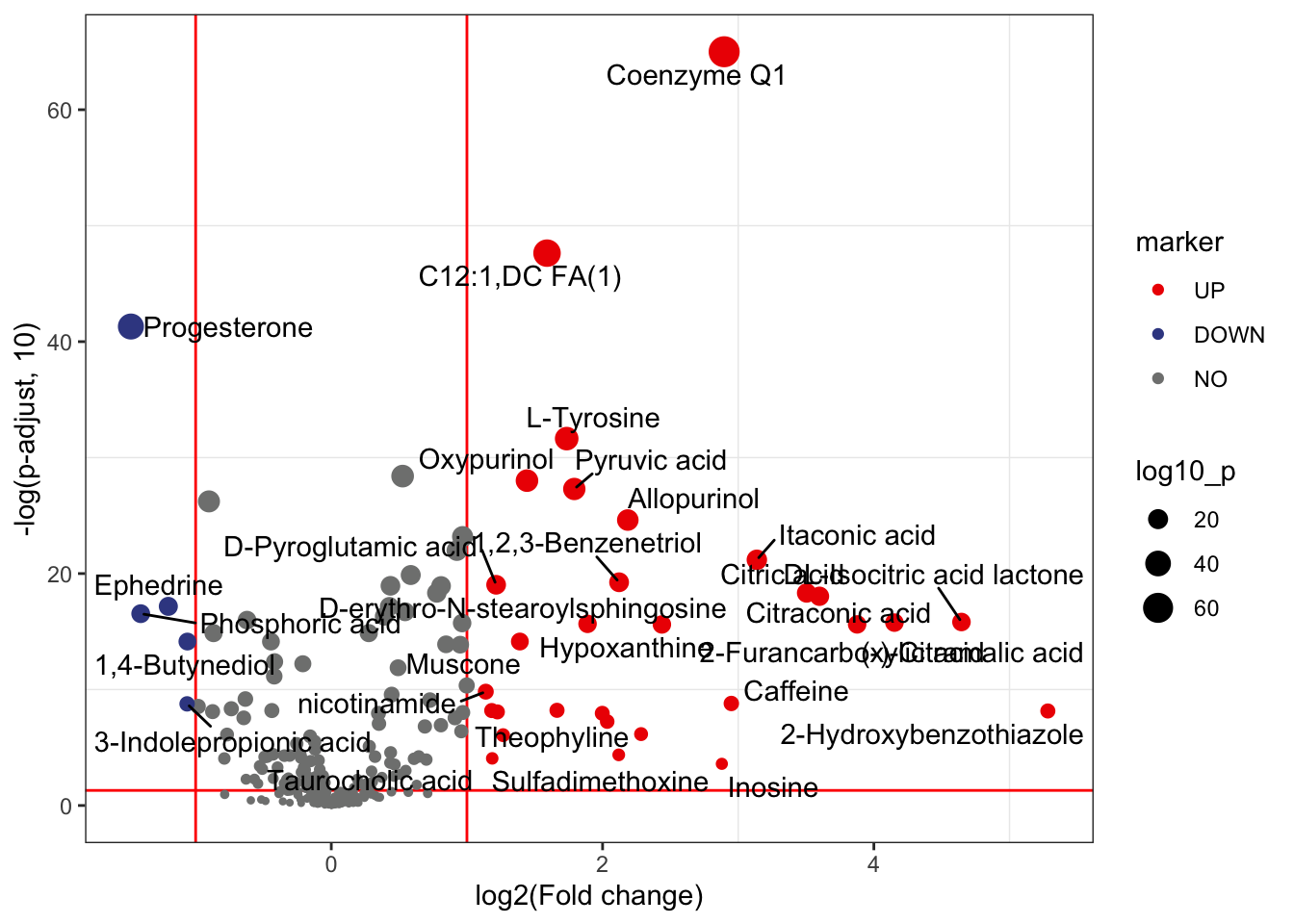
假设存在Case2,绘制火山图。
1
2
3
4
5
6
7
8
9
10
11
12
13
14
15pdf(file="statistical_analysis/Volcano2.pdf")
p<- volcano_plot(object = object,
fc_column_name = "fc_case2_vs_control",# 重命名后
p_value_column_name = "p_value_adjust_case2_vs_control",# 重命名后
fc_up_cutoff = 1,
fc_down_cutoff = 1,
p_value_cutoff = 0.05,
add_text = TRUE,
text_from = "Compound.name",
point_size_scale = "p_value_adjust_case2_vs_control") # 重命名后
p + scale_size_continuous(range = c(0.5, 5))
dev.off()
保存结果
保存差异表达代谢物结果。如果有多个实验组,则将下述代码中的“fc”和“p_value_adjust”更改为重命名后的名称,并分别保存到不同的文件中。
1
2
3differential_metabolites <- extract_variable_info(object = object) %>% filter(fc > 2 | fc < 0.5) %>% filter(p_value_adjust < 0.05)
readr::write_csv(differential_metabolites, file = "statistical_analysis/differential_metabolites.csv")保存结果对象
1
2
3object_final <- object
save(object_final, file = "statistical_analysis/object_final")
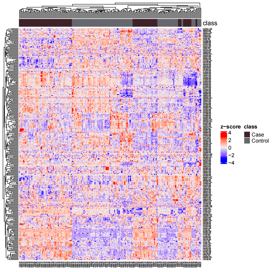
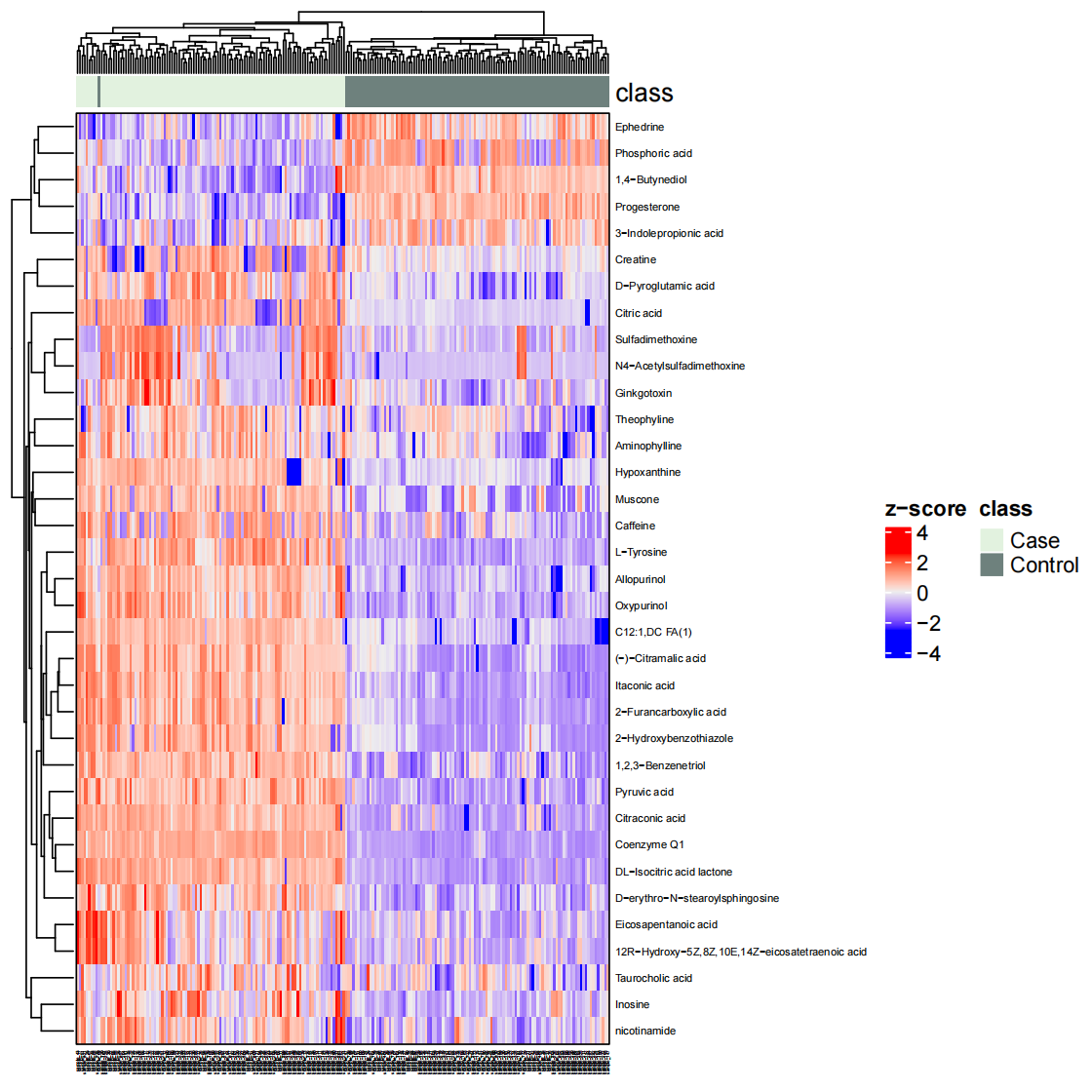
绘制热图
1 | temp_object <- object_final %>% |
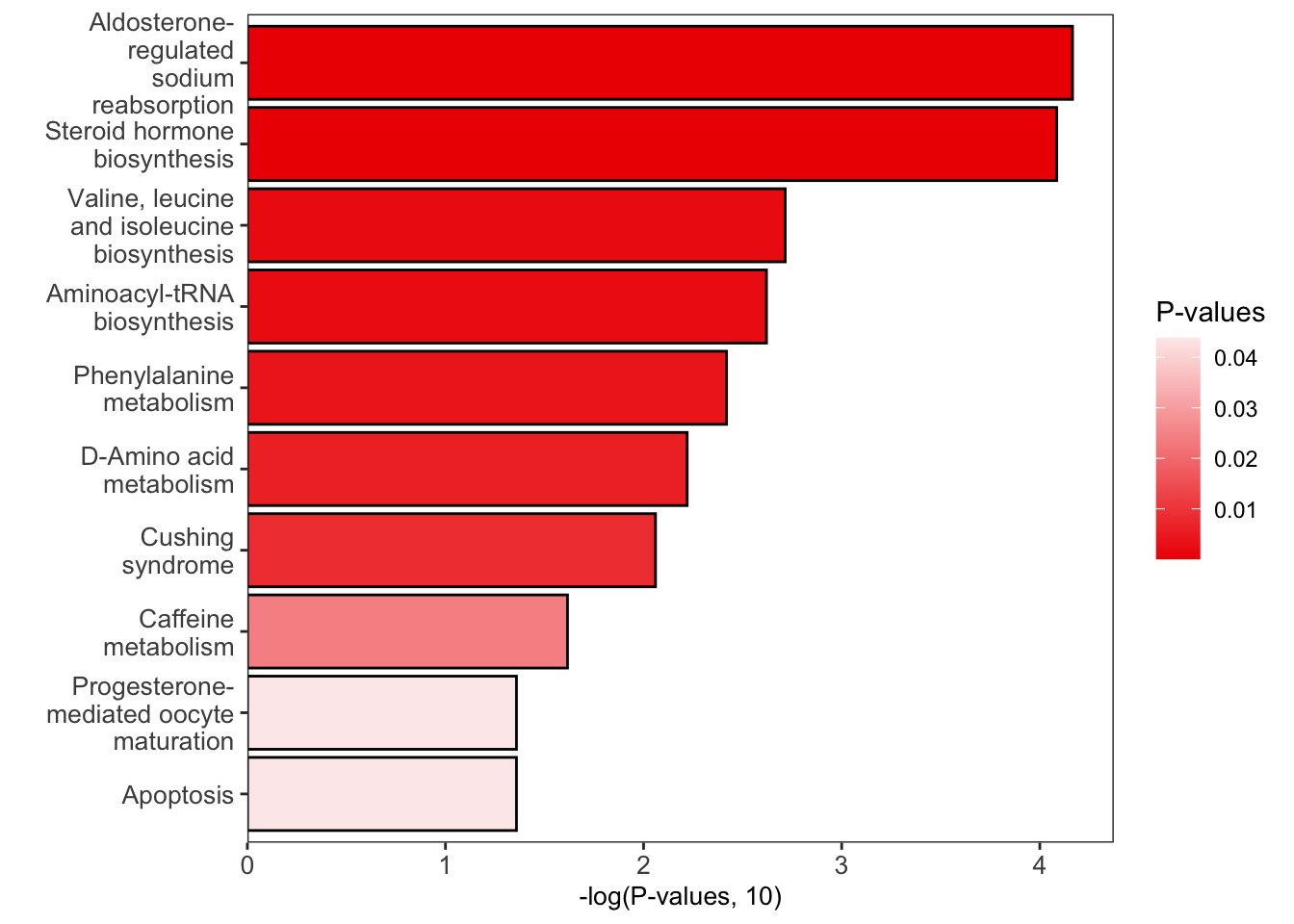
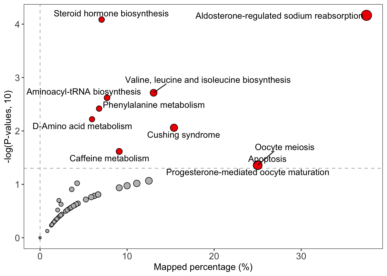
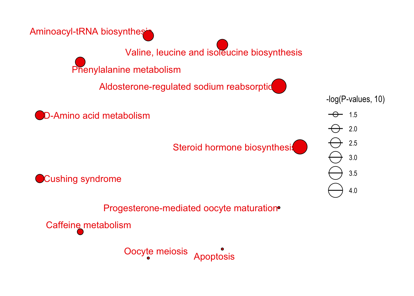
代谢通路富集
导入数据
1 | library(tidymass) |
富集
1 | dir.create(path = "pathway_enrichment", showWarnings = FALSE) |
加载KEGG human pathway数据库
可选数据库:kegg_hsa_pathway,keggMS1database,query_id_kegg,hmdb_pathway,hmdbMS1Database,query_id_hmdb。
??这些数据库的区别是什么?
1 | data("kegg_hsa_pathway", package = "metpath") |
绘制结果
1 | # bar plot |
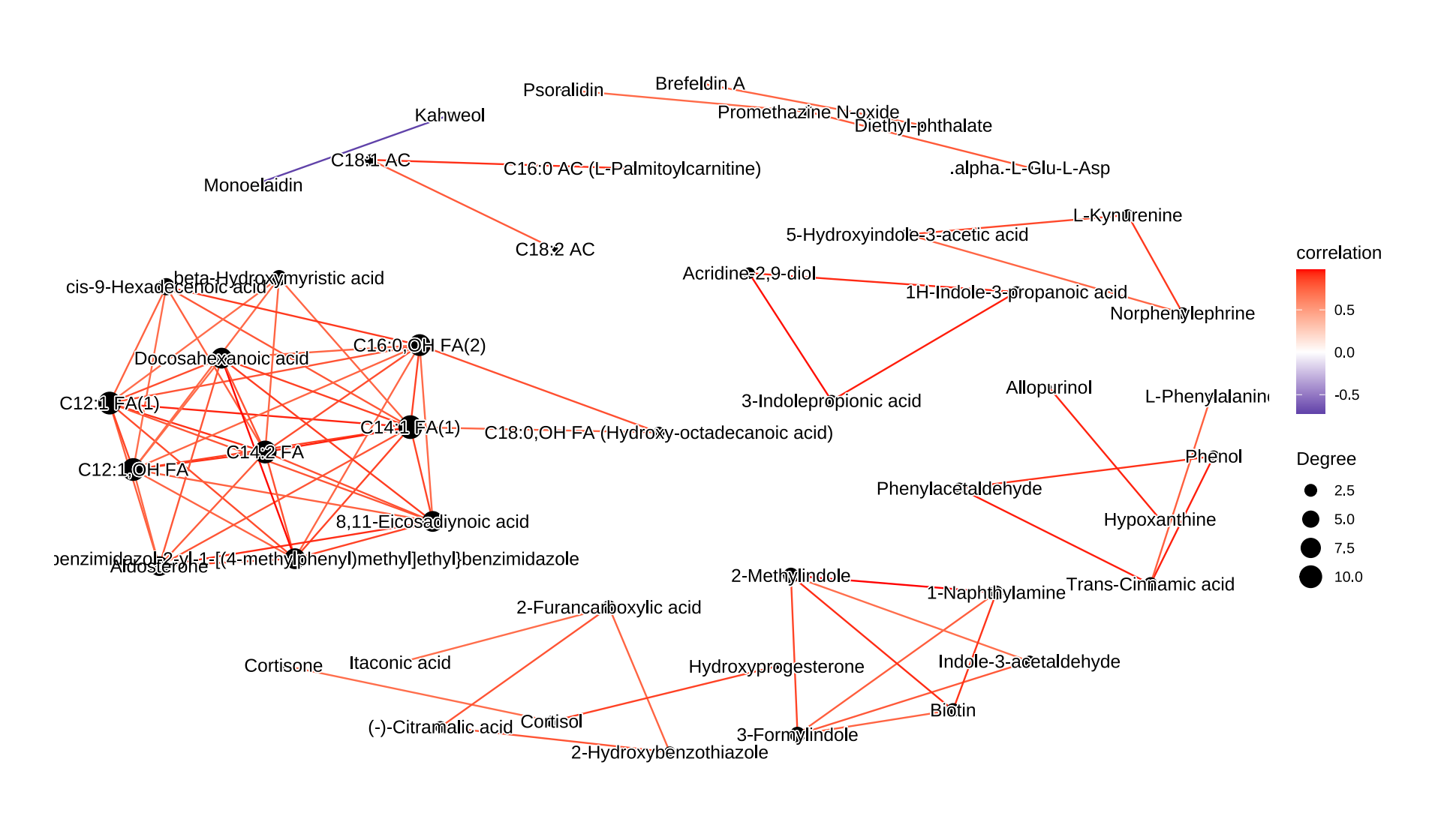
Correlation network analysis
1 | temp_object <- object_final %>% |
术语
- HILIC(亲水相互作用色谱)& RPLC(反相色谱):RPLC 色谱柱主要使用非极性固定相(C18、C8 等),而 HILIC 色谱柱则使用极性固定相(二氧化硅、酰胺等)。两种技术采用的流动相通常由乙腈和水组成,这使得两种液相色谱模式之间可以实现轻松切换。HILIC 和 RPLC 流动相的主要区别在于溶剂洗脱强度。对于 RPLC,乙腈是强洗脱溶剂。但对于HILIC,水是强洗脱溶剂。对于 RPLC,得到的色谱图通常是极性分析物到非极性分析物,而 HILIC 则相反。这种相反的洗脱顺序使 HILIC 成为更常用的 RPLC 的一个很好的补充技术。对于极性分析物和离子化分析物尤其如此,它们在 HILIC 模式下的保留时间更长。
参考
加关注
关注公众号“生信之巅”。
 |
 |
敬告:使用文中脚本请引用本文网址,请尊重本人的劳动成果,谢谢!